Multi-View Stereo Photogrammetry Pipeline - Detailed Algorithm

In my line of work, there are moments when “good enough” simply isn't. When the task at hand is reconstructing a human face in three dimensions with sub‑millimetre precision, every pixel, every algorithmic decision, matters. For years, our team relied on a professional‑grade photogrammetry system, impressively sophisticated, but now a relic of its prime and long abandoned by its manufacturer. I could have treated its decline as an inconvenience. Instead, I treated it as an excuse to pull the machine apart conceptually and learn how it really thinks. That curiosity snowballed into a deep dive through the guts of computer vision where algorithms, statistical models, and mathematical optimizations weave together in a choreography that turns ordinary photographs into finely detailed 3D meshes.

This post is the field notes from that journey: my own 23‑step, six‑phase reconstruction pipeline. Not the manufacturer's playbook, mine, rebuilt from the ground up, the way I understood it, implemented it, and made it work.

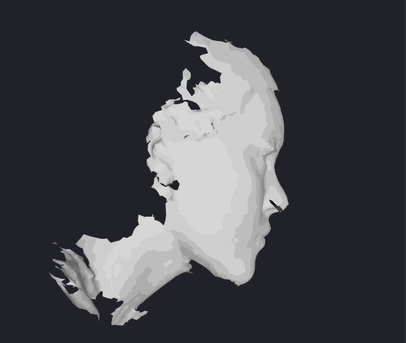
A complete 3D facial reconstruction generated from six synchronized camera views.

Between you and me, this post is already a monster. I apologize but step‑by‑step images will have to wait for the sequel. Took a long time to pin down the details, longer still to write it out.

Phase 1: Camera Calibration and Setup

❮❯⟫⟪

The 3D reconstruction process begins with these six synchronized camera captures; four stereo cameras (1A top-left, 1B bottom-left) (2A top-right, 2B bottom-right) and two texture cameras (1C center-left, 2C center-right) working in perfect coordination to capture every detail of the subject's face. Speckle pattern is clearly visible in stereo captures.

A random speckle pattern is projected onto the facial region, transforming the notoriously smooth geometry of human skin into a textured surface rich with correlation features. This active illumination technique dramatically improves depth calculation accuracy by providing artificial texture where natural skin detail would be insufficient for reliable stereo matching.

Step 1: Parse Camera Calibration Files

Each camera generates a proprietary calibration file containing its complete mathematical mode.

The calibration is based on Tsai's camera calibration method, developed by Roger Tsai at IBM in 1987, but refined over decades of professional use.

Input - Calibration files

Algorithm

1. Parse each file file to extract:
   • 3x3 rotation matrix (M)
   • Translation vector (X, Y, Z)
   • Focal length (f)
   • Principal point (a, b)
   • Pixel size (x, y)
   • Image dimensions (is)
   • Radial distortion coefficients (K, K2)
   • Scale factor (S)
2. Convert Tsai parameters to OpenCV camera matrix format
3. Create distortion coefficient arrays [k1, k2, p1, p2, k3]
4. Store camera poses as 4x4 transformation matrices

Step 2: Validate Camera Configuration

The system performs rigorous checks to ensure all six cameras work together harmoniously.

Algorithm

1. Verify 6 cameras are present (4 stereo + 2 texture)
2. Identify vertical stereo pairs: (1A,1B) and (2A,2B)
   • Note: A1-B1 forms a vertical stereo pair, A2-B2 forms a vertical stereo pair
   • Cameras are arranged vertically to capture different perspectives of the subject
3. Identify texture cameras: 1C, 2C
4. Check calibration consistency across pairs
5. Compute baseline distances between stereo pairs
6. Validate overlapping fields of view

Phase 2: Image Preprocessing and Rectification

Raw camera images require careful preparation before they can be used for stereo matching.

Step 3: Load and Validate Input Images

Input - 6 BMP images per frame

Algorithm

1. Load all 6 images using OpenCV
2. Verify image dimensions match calibration data
3. Check for proper exposure and focus
4. Apply gamma correction if needed for consistent brightness
5. Convert to appropriate data types (float32 for processing)

Step 4: Stereo Rectification

For each vertical stereo pair (1A-1B, 2A-2B)

Algorithm

1. Extract camera matrices K1, K2 from calibration
2. Extract distortion coefficients D1, D2
3. Extract rotation R and translation T between cameras
4. Compute stereo rectification using cv2.stereoRectify():
   • Input: K1, D1, K2, D2, image_size, R, T
   • Output: R1, R2, P1, P2, Q (disparity-to-depth mapping)
   • Note: For vertical stereo pairs, rectification aligns epipolar lines vertically
5. Generate rectification maps using cv2.initUndistortRectifyMap()
6. Apply rectification using cv2.remap()
7. Verify epipolar line alignment (vertical scanlines)

Phase 3: Multi-View Stereo Reconstruction

This is where the real magic happens, transforming 2D image correspondences into precise 3D coordinates.

Step 5: Initialize Stereo Matching Parameters

Based on stereo matching configuration, the system configures critical parameters that control reconstruction quality.

Algorithm

1. Set seed parameters:
   • seed_xmin, seed_xmax: -300 to 300 (search volume bounds)
   • seed_ymin, seed_ymax: -300 to 300
   • seed_zmin, seed_zmax: -300 to 300
   • seedspacing: 80 (initial seed point spacing)
2. Set patch parameters:
   • fixedpatchdiameter: 16 (correlation patch size)
   • adaptive: 0.85 (adaptive patch ratio)
3. Set quality thresholds:
   • precisionlimit: 0.35 (sub-pixel precision threshold)
   • maxskewerror: 0.35 (maximum geometric error)
   • seedchi2sigmalimit: 200 (chi-squared test for seeds)
   • growchi2sigmalimit: 1000 (relaxed chi-squared for growth)

Step 6: Seed Point Generation

The algorithm creates a strategic starting point for reconstruction.

Algorithm

1. Generate regular 3D grid in world coordinates within seed bounds
2. Project seed points to all stereo camera pairs
3. Check if projections fall within image boundaries
4. Filter seeds that don't project to valid regions
5. Initialize seed quality scores to zero
6. Store seeds in priority queue for processing

Step 7: Patch-Based Correlation Matching

For each viable seed point, the system performs sophisticated feature matching using Normalized Cross-Correlation (NCC).

Algorithm

1. Project 3D seed to top and bottom images of vertical stereo pair
2. Extract correlation patches (16x16 pixels default):
   • Reference patch centered at projected point in first camera
   • Target patch searched along vertical epipolar line in second camera
3. Compute NCC:
   • Template matching with sub-pixel interpolation
   • Search range based on depth bounds along vertical direction
4. Find correlation peak with sub-pixel accuracy using parabolic fitting
5. Apply adaptive patch sizing if correlation is weak:
   • Increase patch size up to maxpatchdiameter
   • Decrease if too much texture variation
6. Compute multiple correlation scores for robustness

The adaptive approach impressed me most, when correlation is weak with standard patch size, the algorithm automatically enlarges the search window to capture more textural context, ensuring robust matching across different facial regions.

Step 8: Multi-View Consistency Check

Here's where the vertical stereo configuration really shines.

Algorithm

1. For each stereo match, compute 3D point using triangulation
2. Project 3D point to other stereo pair in the overlapping region.
3. Perform correlation matching in second stereo pair
4. Triangulate second 3D point
5. Compute 3D distance between triangulated points
6. Accept match only if distance < precision threshold
7. Store consistency score for each match

This redundancy dramatically improves reliability in the central facial region while maintaining single-pair reconstruction capability for the sides.

Step 9: Statistical Validation (Chi-Squared Test)

Every potential 3D point undergoes rigorous statistical analysis using chi-squared hypothesis.

Algorithm

1. For each potential match, compute residual vector:
   • Reprojection error in all camera views
   • Photometric consistency across views
2. Compute chi-squared statistic:
   • χ² = Σ(residual²/variance)
   • Use pixel noise standard deviation from configuration
3. Apply chi-squared test:
   • Seeds: χ² < seedchi2sigmalimit (200)
   • Grown points: χ² < growchi2sigmalimit (1000)
4. Reject matches failing statistical test
5. Store confidence scores for valid matches

This statistical framework, developed by Karl Pearson in 1900, provides principled separation of signal from noise with mathematically justified confidence levels rather than arbitrary thresholds.

Step 10: Gauss-Newton Sub-Pixel Optimization

The system refines each accepted match.

Algorithm -

1. Initialize 3D point from triangulation
2. Define objective function:
   • Sum of squared reprojection errors across all views
   • Photometric consistency term
3. Compute Jacobian matrix:
   • Partial derivatives of reprojection w.r.t. 3D coordinates
   • Use finite differences or analytical derivatives
4. Iterate Gauss-Newton steps:
   • Compute parameter update: Δp = -(J^T J)^(-1) J^T r
   • Update 3D point: p_new = p_old + Δp
   • Check convergence (iteration limit or residual threshold)
5. Final 3D point with sub-pixel accuracy

Treating reconstruction as non-linear least squares optimization extracts remarkable precision from noisy image data.

Step 11: Seed-and-Grow Region Growing

Starting from validated seed points, the algorithm expands coverage systematically.

Algorithm

1. Sort validated seed points by confidence score
2. For each high-confidence seed:
   • Add to "grown" point set
   • Mark as processed
3. For each grown point:
   • Find neighboring image pixels (8-connected or 16-connected)
   • Project neighbors to 3D using local depth estimate
   • Attempt correlation matching for each neighbor
   • Apply relaxed thresholds for growth (growchi2sigmalimit)
   • Add successful matches to growth queue
4. Continue until no more points can be grown
5. Apply final consistency check to all grown points

Phase 4: Point Cloud Post-Processing

The multiple stereo pairs generate overlapping point clouds requiring unification.

Step 12: Multi-View Point Cloud Fusion

Sophisticated merging combines data from all stereo pairs.

Algorithm

1. Collect point clouds from all stereo pairs
2. Transform all points to common world coordinate system
3. Identify overlapping regions between point clouds
4. For overlapping points:
   • Compute local point density
   • Merge points within distance threshold
   • Weight by confidence scores
   • Average coordinates and colors
5. Remove isolated points (statistical outlier removal)
6. Create unified point cloud with colors

Step 13: Point Cloud Filtering and Denoising

Algorithm

1. Statistical outlier removal:
   • For each point, find k nearest neighbors
   • Compute distance statistics (mean, std dev)
   • Remove points with distances > threshold
2. Apply bilateral filtering if needed:
   • Preserve edges while smoothing noise
   • Use spatial and photometric distance weights
3. Downsample if point density is too high:
   • Voxel grid downsampling
   • Maintain uniform point distribution

Phase 5: Surface Reconstruction and Hole Filling

Step 14: Surface Mesh Generation

The system creates continuous surfaces from discrete point data using advanced computational geometry.

Algorithm

1. Estimate point cloud normals:
   • Use k-nearest neighbors or radius search
   • Orient normals consistently using MST or viewpoint
2. Apply Poisson surface reconstruction:
   • Set depth parameter based on point density
   • Balance between detail preservation and noise
3. Alternative: Ball pivoting algorithm for unorganized points
4. Extract mesh vertices and triangles
5. Validate mesh topology (manifold check)

Poisson approach frames surface reconstruction as a well-posed mathematical problem rather than ad-hoc triangulation.

Step 15: Hole Detection and Analysis

Even multi-view systems have coverage limitations requiring intelligent gap filling.

Algorithm

1. Compute mesh edges and connectivity:
   • Build edge list from triangle faces
   • Identify boundary edges (edges with only one adjacent triangle)
2. Group boundary edges into contours:
   • Follow connected boundary edges
   • Create closed loops representing holes
3. Classify holes by size:
   • Compute hole perimeter and area
   • Apply maxedgelen threshold from configuration
4. Identify largest hole (assumed to be outer boundary)
5. Mark smaller holes for filling

Step 16: Constrained Hole Filling

Algorithm

1. For each hole to be filled:
   • Extract boundary vertices in order
   • Compute hole center and normal direction
2. Generate internal vertices:
   • Use advancing front technique
   • Maintain edge length constraints (maxedgelen)
   • Ensure good triangle quality (aspect ratio)
3. Triangulate hole interior:
   • Use constrained Delaunay triangulation
   • Respect boundary constraints
   • Optimize for triangle quality
4. Blend with existing surface:
   • Smooth transition at hole boundaries
   • Maintain surface continuity (C0 or C1)

Step 17: Surface Quality Improvement

Multiple filtering passes enhance final mesh quality.

Algorithm

1. Detect surface irregularities:
   • Compute vertex curvatures
   • Identify high-frequency noise
   • Find non-manifold regions
2. Apply smoothing filters:
   • Laplacian smoothing for basic noise reduction
   • Taubin smoothing to preserve volume
   • Bilateral filtering to preserve features
3. Iterate filtering based on ftype parameter:
   • Type 0: Original light smoothing
   • Type 2: More aggressive filtering
4. Validate mesh quality after filtering

Phase 6: Texture Mapping and Final Output

The final phase transforms geometric meshes into photorealistic 3D models.

Step 18: Texture Camera Processing

The two dedicated texture cameras provide high-quality color information.

Algorithm

1. Load texture images (1C.bmp, 2C.bmp)
2. Apply camera calibration corrections:
   • Undistort images using camera parameters
   • Apply color correction if specified
3. Compute texture camera visibility:
   • For each mesh triangle, determine visibility from each texture camera
   • Use ray casting or z-buffer techniques
   • Account for self-occlusion

Step 19: Multi-View Texture Blending

Sophisticated algorithms combine texture information seamlessly.

Algorithm

1. For each mesh triangle:
   • Determine best texture camera based on:
     • Viewing angle (surface normal vs camera direction)
     • Distance from camera
     • Image quality metrics
2. Project triangle vertices to texture camera:
   • Use camera calibration parameters
   • Handle distortion correction
3. Extract texture from source image:
   • Sample texture within projected triangle
   • Apply bilinear/bicubic interpolation
4. Blend textures from multiple cameras:
   • Weight by viewing angle and distance
   • Use Poisson blending for seamless results
   • Handle color differences between cameras

Step 20: UV Mapping and Texture Atlas Generation

Standard parameterization enables compatibility with graphics pipelines.

Algorithm

1. Generate UV coordinates for mesh:
   • Use conformal mapping or angle-based flattening
   • Minimize texture distortion
   • Handle texture seams appropriately
2. Pack UV islands into texture atlas:
   • Optimize atlas utilization
   • Maintain texture resolution consistency
3. Render final texture atlas:
   • Composite multi-view textures
   • Apply final color corrections
   • Generate mipmap levels if needed

Step 21: File Format Conversion

Algorithm -

1. Export mesh geometry:
   • Convert to standard formats (OBJ, PLY, VRML)
   • Write vertex coordinates and normals
   • Write triangle face connectivity
   • Include texture UV coordinates
2. Export texture atlas:
   • Save as standard image format (PNG, JPG)
   • Include material definitions

Phase 7: Quality Control and Validation

Professional systems require comprehensive quality assessment.

Step 22: Reconstruction Quality Assessment

Algorithm

1. Compute reconstruction metrics:
   • Point cloud completeness (coverage percentage)
   • Mesh quality metrics (triangle aspect ratios, edge lengths)
   • Texture quality assessment (blurriness, seam visibility)
2. Generate quality reports:
   • Per-region quality scores
   • Overall reconstruction confidence
   • Identify problematic areas
3. Compare with reference data if available

Detailed analysis ensures results meet accuracy requirements.

Step 23: Final Output Organization

Algorithm

1. Create output directory structure:
   • 3D models (mesh files)
   • Texture files (images and materials)
   • Metadata (calibration, quality reports)
   • Processing logs
2. Generate documentation:
   • Processing parameters used
   • Quality assessment results
   • Reconstruction statistics

❮❯⟫⟪

The reconstructed mesh projected onto subject's face for validation.

The Beauty of Vertical Stereo Architecture

An important point to make here is that vertical stereo pair configuration elegantly solves several challenging problems.

Geometric Advantages:

1. Vertical baselines provide optimal triangulation for facial depth variations
2. Avoids occlusion issues that plague horizontal 3. stereo systems
3. Natural alignment with facial symmetry patterns
4. Superior depth resolution for nose, eye sockets, and cheekbone features
5. Of course if this isn't enough, speckle pattern also helps to provide positive correlation.

Coverage Strategy:

1. Left pair excels at left facial regions
2. Right pair captures right facial areas with high confidence
3. Central overlap provides critical multi-view validation
4. Region growing connects high-confidence areas with single-view regions

Statistical Rigor - Every step applies principled mathematical methods rather than heuristics. The chi-squared validation, Gauss-Newton optimization, and Poisson reconstruction demonstrate decades of algorithmic refinement.

Engineering Excellence

This deep dive revealed that 3D object reconstruction isn't magic (not that it was ever claimed to be), it's carefully orchestrated steps of computer vision, statistical analysis, and mathematical optimization working in perfect harmony. Every millisecond of capture represents thousands of calculations, correlation matching, statistical validation, geometric optimization, and surface reconstruction. The result - millimeter-accurate 3D models from simple photographs, demonstrates the incredible power of well-engineered algorithmic pipelines.

The legacy system that sparked this journey contained decades of refined engineering knowledge. Each of these steps represents solutions to real-world problems discovered and solved through years of professional use.

I'm not going to pretend I understand every algorithm, term, or technique in this pipeline. Engineers decades ahead of me have spent years perfecting the right solutions, the right parameters, and the right workflows. My own path relied on trial and error, a dose of good ole LLM assistance, and my particular flavor of autism helped immensely. At one point, frustrated by the lack of results, I even considered breaking out Ghidra. In hindsight, I'm glad I didn't. The process pushed me to become a better problem‑solver.

And that's really the point. This wasn't just about building a working pipeline, it was about learning how to navigate the unknown. The end result might be code and calibration, but the journey was persistence in its purest form.

I've kept things high‑level here, skipping the step‑by‑step maths for now, but this algorithm should be enough to whet your appetite. And if the stars align and permission comes through… you might just see the reconstruction code out in the wild.

Part of what I could release, I rewrote and is now avaliable at GitHub: 3D Facial Reconstruction and GitHub: 3D Mesh Projector.